
Techniques for multiple right-hand sides
Preconditioning techniques considered (I)
We consider techniques to precondition or improve an existing preconditioner second level preconditioning
Solve
 and extract information
Use
 and extract information
Use
 and ...
...

residuals;
descent directions;
steps;
or other vectors such as eigenvectors of
 ...
...
Preconditioning techniques considered (II)
We study and compare two approaches :
Deflation [Frank, Vuik, 2001].
Limited Memory Preconditioners (LMP): Preconditioners based on a set of A-conjugate directions.
Generalization of known preconditioners: spectral [Fisher, 1998], L-BFGS [Nocedal, Morales, 2000], warm start [Gilbert, Lemar´echal, 1989].
we cover:
Theoretical properties.
Numerical experiments (data assimilation).
Properties
Deflation Techniques
Given
 formed with \cre{appropriate information} obtained when solving the previous system.
Consider the

 .
.Split the solution vector as follows
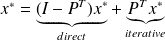 .
.Compute
 with
with
 .
.Compute
 with an iterative method.
Some Properties (Deflation)
Computation of
: Computation of
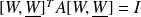
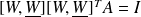
:Any solution} of the compatible singular system
 satisfies
 .
. .
. Use CG with
 to solve
and compute
to solve
and compute
 .
.

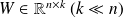
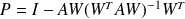
Limited Memory Preconditioners (LMP)


with
 .
.Particular forms
The
 's are the descent directions obtained from CG:
 L-BFGS preconditioner.
The
's are eigenvectors of
:
 spectral preconditioner.
The
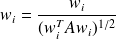
's are Ritz-vectors of
wrt an orthognal basis
 :
:
 Ritz preconditioner.
Spectral Properties for LMP (I)
Fundamental : Theorem
The spectrum
 of the preconditioned matrix
 satisfies} :
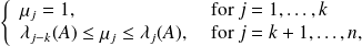
Note: the matrix A to precondition is the same (only the RHS changes).
Proof
Assume that the
 have been normalized, without loss of generality :

with
 . Let
. Let
 , be the
-conjugate complement of
, be the
-conjugate complement of
 . The following conjugacy relations hold :
 .
.
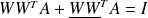
We have
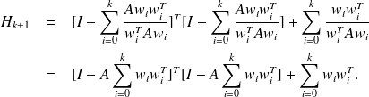 .
.
This can be rewritten in terms of matrices
It can be shown as follows that
 . Using the conjugacy relations, we have
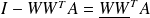
 and since
 , the matrix
 left by
 yields
 which is equivalent to
 .
.
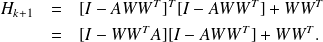
Therefore
 writes
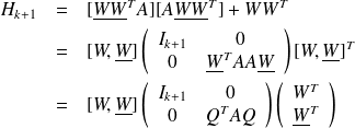
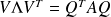
The matrix
 is an orthogonal matrix of
 . Since
 with
with
 , is a spectral decomposition of the matrix
 , we have
 .
.
The matrix
 has the same spectrum as the matrix
and can be written
has the same spectrum as the matrix
and can be written
This is a diagonalization of the matrix
 , because
 is orthogonal. The result follows from (see Horn anf Johnson)
 with
with
 .
.
Spectral properties for LMP (II)
nn
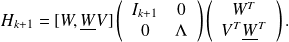
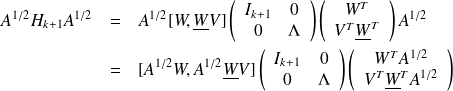
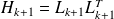
Existence of a factored form for the LMP (not the Cholesky factor !)
L-BFGS :
A
 is
is
 where :
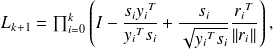
with
 and
and
 .
.Same cost in memory and CPU as the unfactored form.
Spectral :
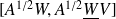
A possible factored form is
 where :
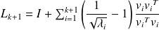
Same cost in memory as the unfactored form.
Why looking for a factored form H = LLT ?
With a non factored form, we use CG preconditioned by H.
With a factored form, we solve
 .
.
 :
:When accumulating preconditioners, symmetry and positiveness are still maintained :

Least-squares
 :
:LSQR (or CGLS) is more accurate than CG in presence of rounding errors but works with
 instead of
 .
.More appropriate if reorthogonalization of the residuals is used.
Experiments with LSQR
LSQR is better than CG !
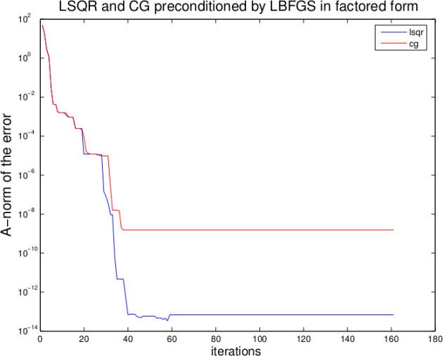
LSQR is again better than CG !
Why to reorthogonalize the residuals ?
In finite precision, residuals often loose}orthogonality (or conjugacy) and theoretical convergence is then slowed down.
Reorthogonalization of residuals in CG is terribly successful} when matrix-vector product is very expensive compared to other computations in CG (see example in the next slide).
Note: to restore orthogonality or conjugacy, working with
 and the canonical inner-product is better (memory, CPU, error propagation) than working on
preconditioned by
and the canonical inner-product is better (memory, CPU, error propagation) than working on
preconditioned by
 .
.
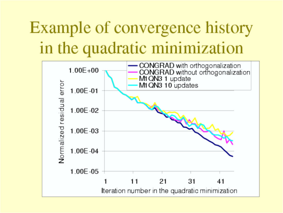
Example of reorthogonalization effect : CERFACS data assimilation system (1 000 000 unknowns)
Experiments
Experiments with a data assimilation problem
Problem formulation : nonlinear least-squares problem

Size of real (operational) problems :
 ,
,

The observations
 are noisy.
Solution strategy : Incremental 4DVAR (i.e. inexact/truncated Gauss-Newton algorithm).
Main ingredients
Sequence of linear symmetric positive definite systems to solve :

Whose matrix varies.
Experiments description
Algorithmic variants tested :
Use CG to solve the normal equations.
Compare with Deflation (spectral) 3 LMP preconditioning techniques :
Ritz technique (
"using Ritz information"
).Spectral preconditioner (
"using spectral info."
).L-BFGS preconditioner (
"using descent directions"
).
Where spectral information is needed, use Ritz (vectors) as approximations of the eigenvectors.
Ritz vectors are obtained by mean of a variant of CG : the Lanczos algorithm which combines linear and eigen solvers.
Experiment large system OPA VAR
OPA ocean general circulation model.
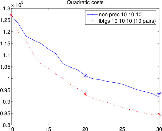
Comparison of the effect on the second quadratic minimization (the first is used to obtain the information).
Comparison of the quadratic/Nonlinear cost. Information : the 10 vectors obtained using the first outer-loop (10 cg steps).
L-BFGS better than no preconditioning
Spectral is worse than no preconditioning
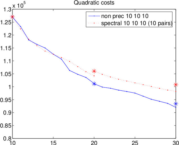
Something strange about deflation
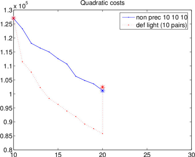
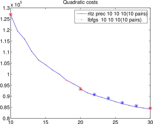
Ritz = L-BFGS for 10 pairs
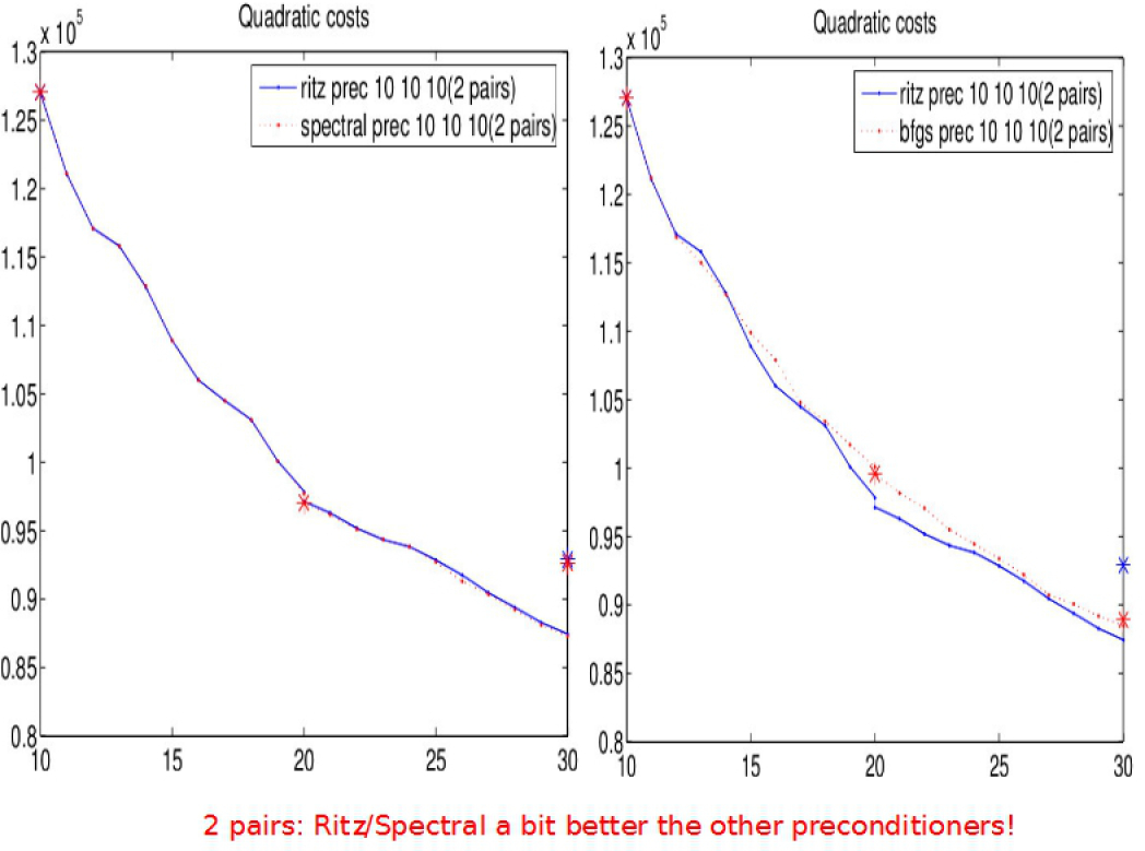
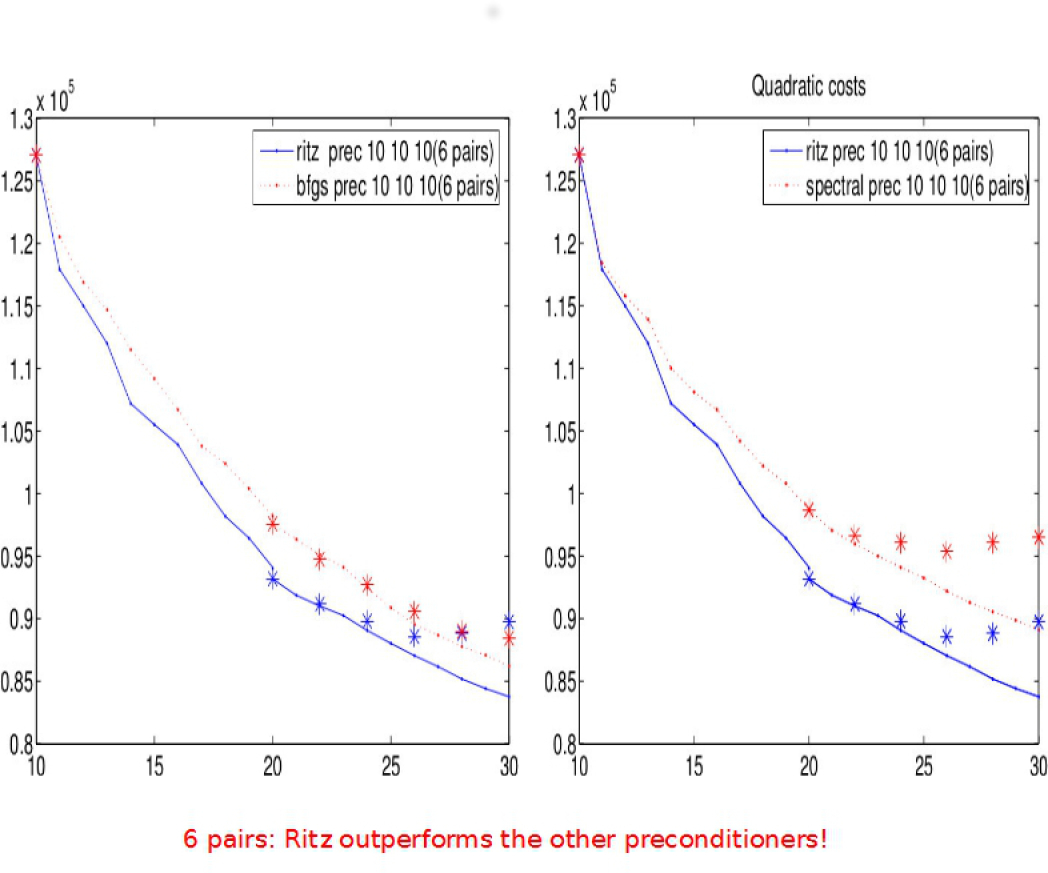
Preconditioner comparison
Comparison with the same number of pair (unfair, memory-wise spectral=bfgs cheaper than deflation=LBFGS)
Number of pair considered : 6 and 2
Remarks on our system !
Spectral preconditioner does not work in our case (
 vectors).
L-BFGS/Ritz preconditioner: (
 )
)Based on by-products of CG.
More efficient than the spectral preconditioner or than no preconditioner.
Ritz is a stabilized version of spectral
Deflation: the computationally ”light” version is not efficient (
 ).
).There is a ”full version” for all the preconditoners : work to prepare the preconditioner not neglectable, but robust wrt large matrix changes. The full form are being compared. They all have the same cost. Usefull when starting a system with poor initial guess. versions of the Ritz/Spectral/L-BFGS that do have the same property (and unfortunately cost). Usefull when starting a system with poor initial guess.


