The SPD case
The conjugate gradient method
The Ritz-Galerkin approach
The condition
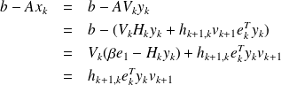
 can be written
 .
.
Using
 we have
 .
.
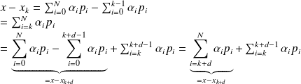
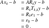
Because
 and
and
Note that
 is a by product of the algorithm.
If
 is symmetric,
 reduces to a tridiagonal
 .
.
Fundamental : Proposition 3
Because
is SPD, the bilinear form
 defines an inner product.
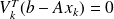
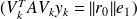
The Ritz-Galerkin condition
 can be written
 which also reads
 .
.
This latter condition implies that
 is minimal over
The Lanczos algorithm
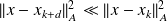
In the Ritz-Galerkin approach the new residual
 is orthogonal to
 such that
 is colinear to
 .
.
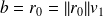
Since from
 . We can relax the normalisation constraints on the
 such that
 .
.
Because
 there exists a polynomial
 of degree
 such that
It follows that
 From the
 column of
 we have

Using
 in both sides of

and identifying the coefficient for b we obtain
 which defines the scaling
 enabling to have
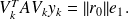
 Denoting
 we have
 , where
 is a tridiagonal matrix with entries

Similarly to the Arnoldi case we also have
Because
 , we have
 .
.
The Ritz-Galerkin condition writes
 , and hence

Using
 we obtain
Because
 is the solution of

Note that for
 the construction of the orthogonal basis mustterminate ; in that case

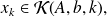
Let
 be the solution of
 then
then
 Indeed,
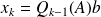
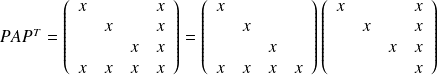
The main drawback of this approach is thet is requires to store
 to build
 from
from
 . Notice that so far we have only use the symmetry property of
 Exploiting the positivness of
leads to a clever variant of the above Lanczos algorithm that is better known as the Conjugate gradient method.
Exploiting the positivness of
leads to a clever variant of the above Lanczos algorithm that is better known as the Conjugate gradient method.
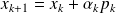
The CG Algorithm
|


Some properties of CG
An upper-bound for the convergence rate
From
 we have that
Then we have
 . In addition,
is minimal over
. In addition,
is minimal over
 .
.
Fundamental : Proposition 4
The polynomial
 built by CG is such that
 ,
,
where
 is the set of polynomial of degree
 .
.
Fundamental : Proposition 5
Let
be the
iterate generated by the CG algorithm then
Proof
From Proposition (4) we have
 .
.
Let
 ,
,
 be the eigenvalues of
and
be the eigenvalues of
and
 where
where
 the components of
 in this eigenbasis
 .
.
We have
 , and
, and
 then
then
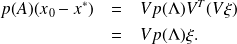
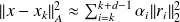
We therefore have that
This shows that

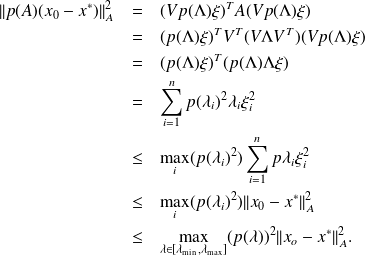
Using an approximation theory result we have

where
 is the Chebyshev polynomial of the first kind of degree
 . For
. For
 we have

Let
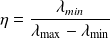 we have
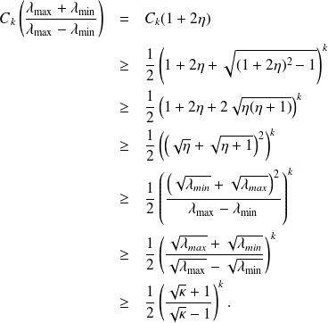
This implies that
 .
.
Plugging this bound in
and then in
completes the proof.
Convergence v.s. the spectrum of A
For symmetric matrices, the degree of the minimal polynomial
is equal to m the number of distinct eigenvalues.
Corollary 28
From Proposition(4) we have
 .
.
This indicates that CG will converge in at most $m$ iterations for any initial guess
 .
.
Coollary 29
If
 has
components in the eigenbasis, CG will converge in
iterations.
has
components in the eigenbasis, CG will converge in
iterations.
CG v.s. the A-norm of the error
Fundamental : Proposition 6
The CG iterates are such that
 .
.
he A-norm of the error is decreasing, if
 is such that
then
 .
.
Proof
In the CG algorithm, the vectors
 are conjugate wrt to
. Remember
are conjugate wrt to
. Remember
 . Let
. Let
 be the solution
 .
.
The result follows easily from the Pythagore Theorem with inner product
on the expression