
Iterative solvers
Introduction
Alternative to direct solvers when memory and/or CPU constraints.
Two main approaches
Stationary/asymptotic method :
 .
.Krylov method :
 subject to some constraints/optimality conditions.
Advantages | Drawbacks |
|
|
|
|
Stopping criteria based on backward error analysis
The error introduced during the computation are interpreted in terms of perturbations of the initial data, and the computed solution is considered as exact for the perturbed problem. The backward error measures in fact the distance between the data of the initial problem and those of the perturbed problem. Let
 be an approximation of the solution
 . Then
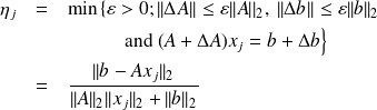
is called the normwise backward error associated with
. If perturbations are only considered on
 or if
or if
 is unknown
we can also consider

Notice that if
 this reduces to a stopping criterion finds in many codes/papers.
Stationary methods
Basic scheme
Let
 be given and
 a nonsingular matrix, compute

Note that
 the best
 is
is
 .
.
Fundamental : Theorem
The stationary sheme defined by

converges to
 for any
if
for any
if
 , where
 denotes the spectral radius of the iteration matrix
 .
.
Some well-known schemes
Depending on the choice of
we obtain some of the best known stationary methods.
Let decompose
 , where
 is lower triangular part of
 ,
,
 the upper triangular part and
 is the diagonal of
.
is the diagonal of
.
 : Richardson method,
 : Jacobi method,
 : Gauss-Seidel method.
Notice that
has always a special structure and inverse must never been explicitely computed.
 reads solve the linear system
 .
.
Krylov methods
Krylov methods: Motivations
For the sake of simplicity of exposure, we assume
.This does not mean a loss of generality, because the situation
 can be transformed with a simple shift to the system for
which obviously
 . The minimal polynomial
 of
is the unique monic polynomial of minimal degree such that
of
is the unique monic polynomial of minimal degree such that
 .
.
It is constructed from the eigenvalues of
as follows. If the distinct eigenvalues of
are
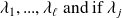 has index $m_j$ (the size of the largest Jordan block associated with
 ), then the sum of all indices is

When
is diagonalizable
 is the number of distinct eigenvalues of
; when
is a Jordan block of size
is the number of distinct eigenvalues of
; when
is a Jordan block of size
 , then
 .
.
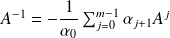
If we write
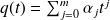 , then
the constant term
 .Therefore
 if
is nonsingular. Furthermore, from
if
is nonsingular. Furthermore, from

it follows that
 .
.
This description of
portrays
 immediately as a member of the Krylov space of dimension
associated with
and
denoted by
immediately as a member of the Krylov space of dimension
associated with
and
denoted by
 .
.
The Krylov subspace approach
The Krylov methods for identifying
 can be distinguished in four classes :
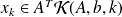
The Ritz-Galerkin approach :
construct
 such that
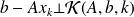 .
.The minimum norm residual approach :
construct
such that
 is minimal
The Petrov-Galerkin approach :
construct
such that
 is orthogonal to some other
 -dimensional subspace.
The minimum norm error approach :
construct
 such that
is minimal.
such that
is minimal.
Constructing a basis of K(A, b, k)
The obvious choice
 is not very attractive from a numerical point of view since the vectors
 becomes more and more colinear to the eigenvector associated with the dominant eigenvalue. In finite precision calculation, this leads to a lost of rank of this set of vectors.
A better choice is to use the Arnoldi procedure.
The Arnoldi procedure
This procedure builds an orthonormal basis of
 .
.
|


The Arnoldi procedure properties
Fundamental : Proposition 1
If the Arnoldi procedure does not stop before the
 step, the vectors
 form an orthonormal basis of the Krylov subspace
 .
.
Proof
The vectors are orthogonal by construction.
They span
follows from the fact that each vector
 is of the for
 , where
 is a polynomial of degree
 . This can be shown by induction.
For
 is is true as
 with
with
 .
.
Assume that is is true for all
 and consider
 .
.
We have

This shows that
can be expressed as
 where $
 is of degree
.
is of degree
.
Fundamental : Proposition 2
Denote
 the
the
 matrix with column vector
 ;
;
 the
the
 Hessenberg matrix whose nonzero entries are
 and by
 the square matrix obtained from
by deleting its last row. Then the following relations hold :
the square matrix obtained from
by deleting its last row. Then the following relations hold :
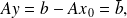
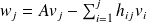
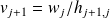
Proof
The relation
 follows from the equality which is derived from step 4, 5 and 7 of the Arnoldi's algorithm.
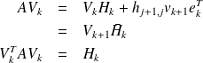
If we consider the
 column of
 , i.e.
 ...
...

This relation holds for all
 . Relation
 is a matrix formulation of
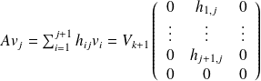 .
.
It is derived from
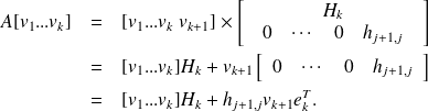
Relation
 mainly exploits the orthogonality of
 .
.


