
Gradient computation
We have seen that data assimilation leads to optimization problems.
Gradient based optimization is often required to solve large problem. The alternative is ”derivative free” optimization, which may not be suitable to large problems.
Algorithms to compute the gradient of the 4D Var functional are needed.
Practical computation of the gradients
Very intuitive : finite differences
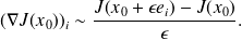
Problem : CPU Expensive, choice of

Direct use of the previous slides: store matrices
 and
and
 and implement the formulas.
Problem: Memory Expensive.
rator based approach: implement the operations
 ,
,
 . This is the right approach for large problems.
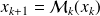
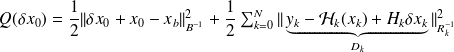
The problem considered is
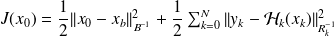
with
 . By differentiating this expression, we get from the chain rule

where
 .
.
This yields
 .
.
Using a Horner-like scheme, we write
 .
.
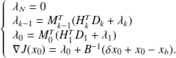
Therefore, for

 can be evaluated by the backward recursion
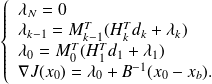
and for the gradient of the quadratic problem
 ,
,
we get
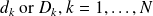
Computation of the gradients
and
 requires
Computation of
 : Integration of the dynamical system.
Computation of the misfits
 .
.Computation of the so-called adjoint variables

Notes
For a given quadratic
 , only steps
 . and
. and
 . are needed to compute
.
. are needed to compute
.To compute
 , evalutation
 needed :
application of the operator representing the adjoint of the tangent of the linear model.
Operator differentiation. Use programs to compute
the devivatives of a code
the adjoint of a code.
Automatic differentiation takes a program as input and generates a the code implementing the derivative (tangent) or the transpose of the tangent (adjoint) as output.
It can be used for higher order differentiation
In CPU, computing the derivative of a function costs a few times the cost for the function evaluation.
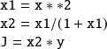
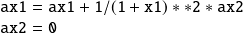
Example :
Consider
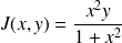 . We want to compute
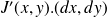
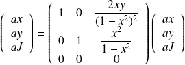
The direct code reads | The tangent code reads (forward mode) |
|
|
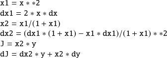
Automatic Differentiation (an introduction)
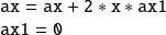
The automatic differentiation tool translate the direct code, routine by routine and line by line, into the tangent
code. For the adjoint code, it is convenient to express the operations in terms of matrices. The tangent linear
operation
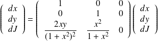
the adjoint operation is
|
|
| |
|
|
|
|

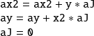
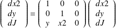
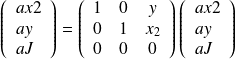


The gradient is obtained when the computation is initialized with
 and
and

Direct/reverse mode
When applied to a mapping
 , the direct code computes
 (directional derivative). Obtaining the gradient of a scalar function costs at least
 times the cost of the function evaluation.
Applied to a scalar function
, the reverse mode gives the gradient and costs a few times the cost of a function evaluation. Applied to a general mapping
, it enables the computation of
 . The main difficulty associated with the reverse mode is the memory mangement (storage of a tree).
Important queston related to the sparsity of Jacobian and Hessian to better optimize the computation.
Popular codes are ADIFOR, ADIC, ADOL-C.
These tools are not "magic" : role of round-off errors, of dicretization errors, pathological "if then else" structures. The user has to think about differentiability issue and stability of the computation.


