
Solution algorithms
Newton method
Depends on the problem size. for reasonable size problems (machine?) it requires the solution of

It converges locally quadratically to a critical point
 under some assumptions (
 is Lipschitz continuous around
and
is Lipschitz continuous around
and
 is SPD)
It is possible to make the convergence global under mild assumptions with trust-region techniques. Linesearch is also possible.
If feasible (size, computational cost) this is a method of choice.
Impraticable for the ocean and atmosphere data assimilation problems.
Quasi-Newton Method
Several variantis available (SR1, PSB, DFP, BFGS,..)
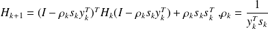
For BFGS, the matrice
is not computed, but its inverse
 is approximated using the secant equation :
The matrix
 is the closest matrix to
for some weighted norm
is the closest matrix to
for some weighted normUpdating formula
Limited memory implementation :
is kept in factored form and only the last pairs are taken into account
 . Example : L-BFGS, M1QN3.
Quasi-Newton method for data assimilation
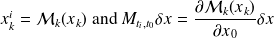
Gradient computation
 ,
, and
and
 are the jacobian matrices of
 and
and
 at
at
 and at
Computing, storing at all step
is not feasible in large scale data assimilation
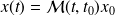
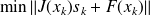
The Gauss-Newton algorithm
Solution of a sequence of linear least squares problems
 and update

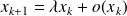
It can be seen as a stationary iteration

Does not require second order information. The linear least-squares problem can be solved by a direct or an iterative method (truncated Gauss-Newton method).
Local convergence of stationary iterations
Definition :
The process
 is locally convergent to
 , if there exist
 such that any sequence
 generated by (
 ) converges to
whenever
) converges to
whenever
 . In this case,
is called a point of attraction.
. In this case,
is called a point of attraction.
If
is a point of attraction of (
) and if
 is continuous at
, then
is continuous at
, then
 , that is,
is a fixed point of
, that is,
is a fixed point of
In the case where
is a fixed point of
, but not a point of attraction of (
), the sequence
may behave in a variety of ways: it may diverge, cycle, or even exhibit a chaotic behaviour.
Ostrowsky's sufficient convergence condition
Let
 ,
,
 , and
, and
 . We denote by
 the identity matrix of order
 .
.
It is well known that, if
 ,
converges to
,
converges to
 for any
. In particular,
is a point of attraction of (
).
for any
. In particular,
is a point of attraction of (
).
Generalization of this result in the case where $G$ is no longer a linear mapping:
Fundamental : Theorem
Suppose that
 has a fixed point
, that
has a fixed point
, that
 is Fréchet differentiable at
, and that
is Fréchet differentiable at
, and that
 .
.
Then
is a point of attraction of the iteration (
).
Asymptotic speed of convergence
Let
be a fixed point of
. Let
 be the set of all of the sequences
generated by (
) and that converge to
.
be the set of all of the sequences
generated by (
) and that converge to
.
Fundamental : Theorem
Suppose
and
satisfy the assumptions of Theorem
 . For
. For
 , one has

Moreover, for any
and
 , there exists a norm
 such that
 for k large enough.
Remarks on Ostrowsky Theorem
he quantity
 is referred to as the root convergence factor of the sequence
,
is referred to as the root convergence factor of the sequence
,converging to
. It can be shown (Ortega, Rheinboldt) that the root convergence factor does not depend on the norm chosen on
 .
.Theorem (
 ) shows that, if
, for any sequence
generated by (
)
) shows that, if
, for any sequence
generated by (
) that converges to
and for any
 such that
 , there exists
 such that
Therefore, the convergence of
 is as rapid as a geometric progression of rate
 .
.Using the norm
 of Theorem (
) , there exists
of Theorem (
) , there exists
 such that
 that is,
converge linearly to
.
that is,
converge linearly to
.Using Theorem (
), for
large enough, the smaller
 , the faster the error
 decreases as
increases.
decreases as
increases.Therefore, if
and
satisfy the assumptions of Theorem (
), the quantity
can be used to measure the asymptotic speed of the convergence of the stationary iteration
 .
.
Local convergence and linear rate of convergence
We denote by
 the Hessian matrix of the function
 .
.
Let

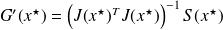
We define
 by
by
Obviously,
is a fixed point of
if
 .
.
The following theorem of local convergence holds :
Fundamental : Theorem
If
 is a fixed point of
,
is a fixed point of
,
 is twice continuously Fréchet differentiable in a neighborhood
 of
,
of
,
and that
 has full rank
. If
has full rank
. If
 , then the Gauss-Newton iteration converges locally to
.
, then the Gauss-Newton iteration converges locally to
.
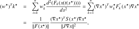
Proof
A direct computation of
 reveals that
 .
.
Let us denote by
 the surface in
 given by the parametric representation
 .
.
The fixed point condition
 has the geometrical interpretation that follows.
let
 be the point of
of coordinates
be the point of
of coordinates
 and
and
 the origin of the coordinate system.
The vector
 is orthogonal to the plane tangent through
to the surface
.
is orthogonal to the plane tangent through
to the surface
.
Fundamental : Theorem
Suppose that the assumptions of the previous Theorem hold and
is nonzero.
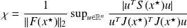
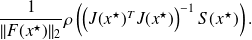
One has
 ,
,
where
 is the maximal principal curvature of the surface ${\cal{S}}$ at point
with respect to the normal direction
is the maximal principal curvature of the surface ${\cal{S}}$ at point
with respect to the normal direction
 .
.
Proof
We consider a curve
 through
on the surface given by the parametric representation
through
on the surface given by the parametric representation
 , and let
 be such that
 . The intrinsic parameter
 on the curve
satisfies
on the curve
satisfies
 ,
,
where
 . The curvature vector of the curve at
is by definition
. The curvature vector of the curve at
is by definition
 . Using the chain rule, yields
Again, the chain rule enables to obtain

The maximal principal curvature of the surface
at point
with respect to the normal direction
 is by definition the supremum over all the curves on
passing through
of the scalar product
is by definition the supremum over all the curves on
passing through
of the scalar product
 .
.
Since
is a fixed point of the iterations,
 , therefore,
were we have denoted by
 the quantity
 . The searched supremum is
and matrix manipulations show that this quantity is equal to
Local convergence properties of the Gauss-Newton algorithm
The algorithm is not globally convergent. It is not locally convergent either : for some problems, a fixed point may be a repelling fixed point.
Consider
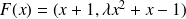 .
.The unique local minimum is
 .
.It is possible to show that
 .
.Therefore, if
 ,
,
 is a repelling fixed point.
Example of nonlocal convergence of Gauss-Newton
The incremental 4D Var algorithm (Gauss-Newton)
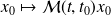
Take

For {
 } solve iteratively the quadratic minimization problem
 , with
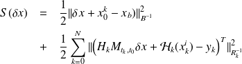
Update
End for
where we set
 .
.


