
Kalman's Filter: II covariance diagnosis and evolution
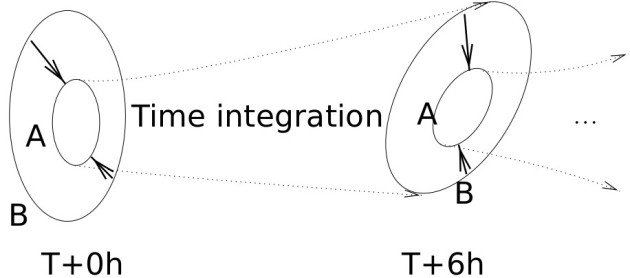
To simplify This dynamics of information one can keep in mind the following simple scheme that mimic pdf evolutions
At a given time
 , in the expression
where
we understand that since the
 matrix is at in first place, it is this matrix that spread into the background
 the correction comming from the innovation
 .
.
Let see an example of such a
matrix and its consequences in terms of assimilation of observations.
First, we introduce a covariance matrix
Some definition that help to feature a covariance matrix:
Definition :
The variance field is the diagonal of the
matrix.We denote by
 the diagonal matrix composed by the square root of the variance field. This is the standard-deviation field.
The correlation functions that are the columns of the matrix
 .
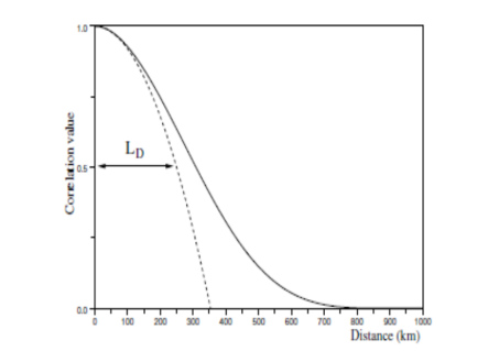
.The length-scale is the characteristic length that feature the degree of correlation between points.
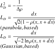
Length-scale definition
More precisely, one can defined the length-scale from the local correlation functions
 as follow [Dal91, PBD08]
 |
(B\&B) |
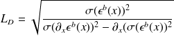
Example : Example of lenght-scale field for the 1D example:
What's happend when we assimilate the same pattern of observation at diffrent places?
Example : Example with Scilab (equivalent to Matlab but free) for the linear dynamic, on the circle,
so that
 the time space.
// Dimension of phase space. n=200; // Geographical position. x=linspace(0,360,n); // Initialization for graphical rep. rect=[0 -1/2 360 1]; nax=[2 5 2 4]; // Definition of the model. c=zeros(n,1);c(2)=1; r=zeros(1,n);r($)=1; M=toeplitz(c,r); | 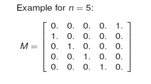 |
Time evolution of a signal.
// Initilization of the signal s=zeros(n,1); s(1:3)=[1/2 1 1/2]'; sn=s; // Loop of time evolution for t=1:100 // Time evolution snp=M*sn; // Graphical representation. clf; plot2d(x,snp,rect=rect,nax=nax); xpause(2000); // Updating of vectors. sn=snp; end |  |
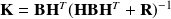
Creation of a
matrix
// Initilization of a B matrix // Initialization of the length-scale dx=x(2);L=4*dx; // Gaussian correlation g=exp(-0.5*(x-x($/2)).^2/L**2)'; // Creation of B nmax=find(g==max(g)); c=[g(nmax:$) ; g(1:nmax-1)]; r=c'; B=toeplitz(c,r); // Graphical representation of some correlations. clf; xset("colormap",jetcolormap(128)); plot2d(x,B(:,1:10:$),rect=rect,nax=nax); | 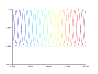 |
Definition :
Definition of the data network and the observational error covariance matrix R, and H the observational operator:
// Data network iobs=n/4:3:3*n/4; p=length(iobs); xobs=x(iobs); R=sigo**2*eye(p,p); plot2d(xobs,zeros(xobs)-0.25,rect=rect,nax=nax,style=-2); H=zeros(p,n); for i=1:p H(i,iobs(i))=1; end | 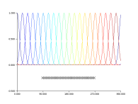 |
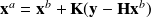
Example : Example of data assimilation and dynamics of information thanks to the Kalman's filter equations
Background - Analysis -Observations
// Example of covariance dynamics I=eye(B); xt=rand(n,1,'normal'); xb=xt+rand(xt,'normal'); for t=1:100 // -- Observation of xt (synthetic obs.) y=H*xt+rand( H*xt,'normal')*sigo; // -- Analysis step K=B*H'*inv(H*B*H'+R); xa=xb+K*(y-H*xb); A=(I-K*H)*B; // PLOT // -- Forecast step xb=M*xa; xt=M*xt; B=M*A*M'; // PLOT B + diag Lp. S=diag(sqrt(diag(B)));iS=inv(S);C=iS*B*iS'; rhop=sum(M.*C,'c'); Lp=1 ./ sqrt(2*(1-rhop)); end |  |
Example : Example of data assimilation and dynamics of information thanks to the Kalman's filter equations
Covariances of
at time q > 1.
// Example of covariance dynamics I=eye(B); xt=rand(n,1,'normal'); xb=xt+rand(xt,'normal'); for t=1:100 // -- Observation of xt (synthetic obs.) y=H*xt+rand( H*xt,'normal')*sigo; // -- Analysis step K=B*H'*inv(H*B*H'+R); xa=xb+K*(y-H*xb); A=(I-K*H)*B; // PLOT // -- Forecast step xb=M*xa; xt=M*xt; B=M*A*M'; // PLOT B + diag Lp. S=diag(sqrt(diag(B)));iS=inv(S);C=iS*B*iS'; rhop=sum(M.*C,'c'); Lp=1 ./ sqrt(2*(1-rhop)); end |  |
Example : Example of data assimilation and dynamics of information thanks to the Kalman's filter equations
length-scale of
at time q > 1.
// Example of covariance dynamics I=eye(B); xt=rand(n,1,'normal'); xb=xt+rand(xt,'normal'); for t=1:100 // -- Observation of xt (synthetic obs.) y=H*xt+rand( H*xt,'normal')*sigo; // -- Analysis step K=B*H'*inv(H*B*H'+R); xa=xb+K*(y-H*xb); A=(I-K*H)*B; // PLOT // -- Forecast step xb=M*xa; xt=M*xt; B=M*A*M'; // PLOT B + diag Lp. S=diag(sqrt(diag(B)));iS=inv(S);C=iS*B*iS'; rhop=sum(M.*C,'c'); Lp=1 ./ sqrt(2*(1-rhop)); end |  |


