Kalman's Filter: I equations
What is this cycle for Gaussian statistics and linear dynamics?
We have to model error. This is done as follow
The prior distribution
 takes the form
 where
where
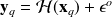
 , the observational operator, mapps the model space
 into the observational space
 ,
,
 is the observational error and we assume it is a Gaussian random variable, centered, and of covariance matrix
 , hence, its distribution is no more than
So what is the plan?
First, we have to detail the analysis step.
then the forecast step
Let start with the analysis step!
analysis step
We apply the Baye's rule within the analysis step, and obtain that
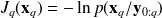
Where
is the likelihood
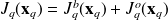
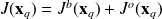
 with
with
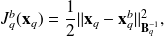
the background term and the observational term
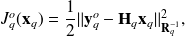
where
 is assumed to be linear, and denoted by
 .
.
In the 1D framework, this corresponds to the scheme
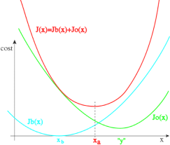
The analysis
 is not too far from the background
 and not too far from the observations

Since
 is quadratic, then it must exists
 and
and
 such that
within a constant (not important due to the normalization).
We have to find
and
:
Due to the quadraticity of cost function
,
is the unique miminum of
, that is the point that nullify the gradient of
.Again, the quadraticity leads that the Hessian of
(that is the second order derivative of
along
 ) is the inverse of the matrix
We find these quantities as follow...
It is easy to find
thanks to the change of variable
 leading to the incremental formulation
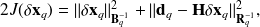
where
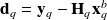 is the innovation.
Then, the gradient of
,
 is null in
 means that
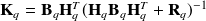
and the computation of the Hessian
 , then its inverse, leads to
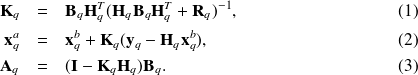
Analysis step
We have obtained that in the Gaussian case, the analysis step provides that
 leads to
with
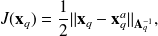
 is a quadratic cost function of unique minimum
where
 and analysis covariance matrix
forecast step
Now we are interested by the forecast step.
By definition,
 is deduced from the time evolution where the linear dynamics implies
Since the linear transform of a Gaussian is also Gaussian, we obtain that the distribution
 is the Gaussian
Where
and

leads to
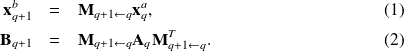
Forecast step
Under linear dynamics and Gaussian distribution, the forecast step provides that
with
and
Hence, for Gaussian distribution and linear dynamics,
Fundamental : Kalman's filter equations
Analysis step:
Forecast step: