
Estimation under the linearity assumption.
Best Linear Unbiased Estimation (BLUE)
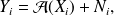
Consider the linear model
 where
where
 is deterministic and
 is a random vector satisfying

Definition :
The
 estimator for
from
estimator for
from
 is the random vector
 which minimizes
 subject to
 and
and

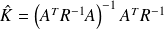
Fundamental : Theorem
If
 has full rank, the BLUE is
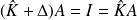
Proof
Starting from
we get
 . This equality should hold for any x, i.e.
 . We have
Set
 , and write
 . From
 , we get

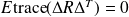
Furthermore,
 and
yields
and
yields
 .
.
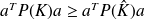
Since
 is positive definite,
 is a scalar product for
 matrices, and
 , if and only if

Optimal Least mean squares estimation I
We consider the random vector
defined by
 where
where
 ,
,
and
is such that

Let us also assume that
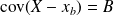
 (uncorrelated pair). For a random vector
 ,
,
we define the error covariance matrix

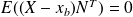
Definition :
The optimal least mean squares estimator
 is such that
 for every matrix
 and every vector
 This variational property is written in short

Optimal Least mean squares estimation II
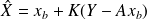
Fundamental : Theorem
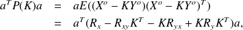
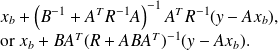
The Optimal Least mean squares is obtained for
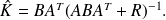
The associated covariance matrix is
 .
.
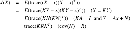
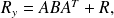
Proof
We set
 then
then
where

Differentiating this expression with respect to
 and setting the derivative to
 gives to

A direct computation shows that
 , which shows that
 is the unique solution.
In addition,

 and
and
 , which shows that
Then
 and the result follows from the Sherman-Morrison formula.
Conclusion
Assume that the random vector
defined by
 , where
 and
is such that
and
is such that
Under various statistical approaches, if the realization
 of
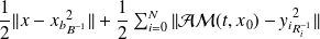
is available, it is reasonable to estimate
as the minimizer of the quadratic functional
of
is available, it is reasonable to estimate
as the minimizer of the quadratic functional
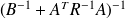
The solution of the problem is unique and can be expressed as
Conclusion : the 4D Var functional
We assume that at

where

 and
and
 is such that
 and
and

We are looking for an estimation of
 that minimizes
The above functional is called the
 functional.
A Data Assimilation experiment I
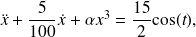
We consider the problem of estimating inital conditions
and
 of the system described by
 from (possibly noisy) observations of

The parameter
 controls the nonlinearity of the problem. For
 , if
, if
 is a particular solution of the problem for zero initial conditions, all the solutions are expressed by

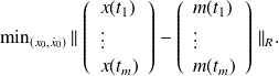
Assume that noisy observations
 of
of
 are available at

We want to minimize the linear least-squares functional
A Data Assimilation experiment II
Solving the linear least squares problem (
)
For each observed quantity
 , computation of the linear theoretical counterpart
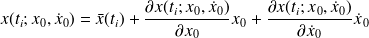
Solution of the linear least-squares problem, using either a direct method (for problem sizes that are small compared to the computer characteristics) or use e.g. a Conjugate Gradient based iterative solver.
We take

Linear case : exact observations (zero noise) v.s. noisy obs.
True trajectory and observations | 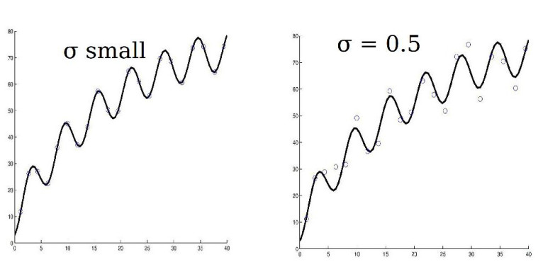 Linear case : exact observations (zero noise) v.s. noisy obs. |
Linear case : exact observations (zero noise) v.s. noisy obs.
True (solid) and estimated (dotted) trajectories | 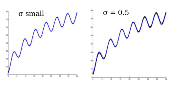 Linear case : exact observations (zero noise) v.s. noisy obs.II |
Values of
 exact
exact
 , no noise
 , and noise

Good forecast even for noisy observations
A Data Assimilation experiment III
Solving the linear least squares problem (
)
Solution based on linearizations of the dynamics around
 Starting point
For each observed quantity
, computation of the linear theoretical counterpart is 
Update

Solution of the linear least-squares problem, using either a direct method (for problem sizes that are small
compared to the computer characteristics) or use e.g. a Conjugate Gradient based iterative solver.
We take
 .
.
Non Linear case : exact observations (zero noise) v.s. noisy obs.
True trajectory and observations | 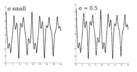 Non Linear case : exact observations (zero noise) v.s. noisy obs. |
True (solid) and estimated (dotted) trajectories | 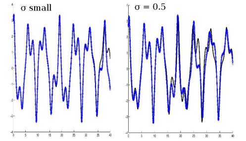 True (solid) and estimated (dotted) trajectories 2 |
Values of
 : exact
, no noise
, and noise
: exact
, no noise
, and noise
Relative bad forecast for noisy observations and
 .
.
Coping with nonlinearity : guess for the analysis
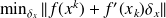
The Gauss-Newton algorithm for
 reads :
 Choose
 , solve
 , update
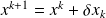 .
.A critical point of
 | is a point where
 .
.In the case of nonlinear least-squares problems, the Gauss-Newton algorithm does not converge from any stating point to a critical point.In the case of nonlinear least-squares problems, the Gauss-Newton algorithm does not converge from any stating point to a critical point.
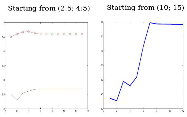
Coping with nonlinearity : convergence histories
Plot the iterates, the solution of the problem without noise is
 Here the noisy problem is considered.
Coping with nonlinearity : residual histories
Plot of the nonlinear least-squares residual

No convergence when the starting point is far from the solution.


