
Estimation under the Gaussian assumption
Definition :
Suppose a random vector
 has a joint probability function
 , where
 is an unknown parameter vector.
Suppose
 is a realization of

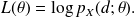
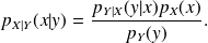
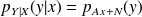
A maximum likelihood estimator for
given d is a parameter that maximizes the log likelihood function
Example :
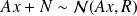
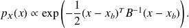
Suppose
 is a realization of a Gaussian vector
 , where the parameter
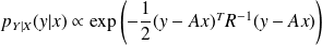
 is unknown. The log likelihood is
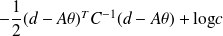 , and
, and
 is the solution of the linear least-squares problem
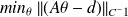 .
.
Some rationale for the maximum likelihood
The information we have is that
is a realization of
. We have (make a picture involving disjoint sets)
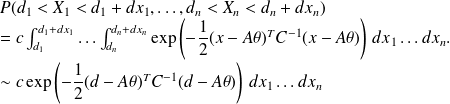
Therefore if
 is enlarged, the probability that
 (i.e. d is close to a realization of
) is increased). Note that
(i.e. d is close to a realization of
) is increased). Note that
 , is equivalent to
 .
.
Inclusion of a priori information on thêta
We may want to incorporate additonal information by viewing the parameter vector
as a realization of a random vector
.This analysis is refered to as Bayesian estimation
It relies on the notion of conditional probability given
 , defined by the function of
 :
:
If
and
 are independant random vectors
Definition :
The maximum a posteriori estimator maximizes
 over
over
 . Is is a function of
Example :
We consider the random vector Y defined by
 where
where
 and
and
 are two independent random vectors.
Let
be a realization of
. The MAP of
is
Proof
The Bayes'law reads
Since
 ,
,
from the independence of
 and
we get
and
we get
 .
.
From
 we get
 .
.
In addition,
 does not depend on
and
does not depend on
and
Therefore, the MAP minimizes
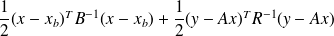
The random vectors are assumed Gaussian. However there might be systematic errors making the estimation unreliable.
Suppose
 and
and
 is nonsingular. Then
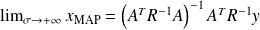 , and we recover the maximum likelihood estimator.
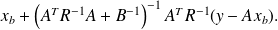
The useful matrix equality (Sherman-Morrison)
 can be used to show that
These two formula are computationally very different when
 is such that
 or
or
 .
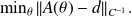
.The maximum likelihood estimation works for nonlinear A and leads to
Proof of (*)
From the SM formula, we get

which yields
 .
.


