
Chaotic behaviour of some fluid
Most of time, physical systems are robust to small disturbance.
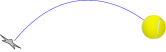
Take a tennis ball.. and its trajectory
Most of time, physical systems are robust to small disturbance.
Little change in the initial condition, little trajectory changes
How do small disturbances evolve with time?
We first consider the solution with initial condition
 . Thanks to the flow, the general solution is

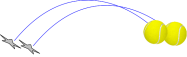
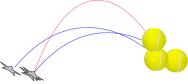
Now, consider a closed initial condition
 This leads to the perturbed solution

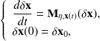
From the Taylor expansion, we obtain

where
 is the propagator associated to the tangent linear model and thus

The propagator
results from the time integration of the dynamics
where
 is the Jacobian matrix of the nonlinear dynamics M, that is it is defined by

Most of time, physical systems are robust to small disturbance.
Little change in the initial condition, little trajectory changes
Most of systems are robust to initial perturbation...
What's about geophysical flow?
In the 1960's, Lorenz was studying the dynamics of nonlinear. It was thought at this time that only a limited number of linear dynamics was required to forecast the weather.
Lorenz was not agree with this point and he tried to show this non-sens from simple dynamics.
He heared of the existence of a nonperiodic dynamics discovered from Galerkin's projection on the lead modes of convection. He has explored it and ...
This is the start of a beautiful story that we'll see later!
Instead of detailling the [?], we explore a geophysical approach for synoptic flow as he has introduced in [?].
For St-Venant Equations,
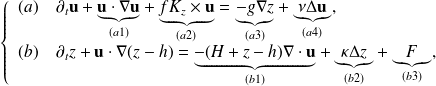
(a) momentum conservation with: nonlinear advection of wind
(a1), coriolis term (a2), pressure term (a3) and dissipation (a4).
(b) interface dynamics with: the divergence term (b1), the
forcing (b3), (b2) simulate thermal dissipation.
Under the small Rossby number approximation, we obtain the QG model
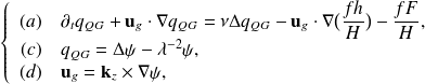
where
 is the Rossby deformation radius.
We chose to project the current function
 onto the smallest number of modes that preserve the nonlinear interaction.
Hence, at least three modes are needed so the verify
We chose the following modes
After the change of variable,
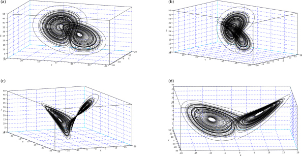
We obtain the Lorenz's system
where the numerical simulation is
Representation in the phase space of mangitudes (X;Y; Z) leads to
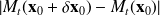
For the Lorenz's model [?], consider two initial conditions
 and
and
 , then compute the time evolution of the distance
 What's happend ?
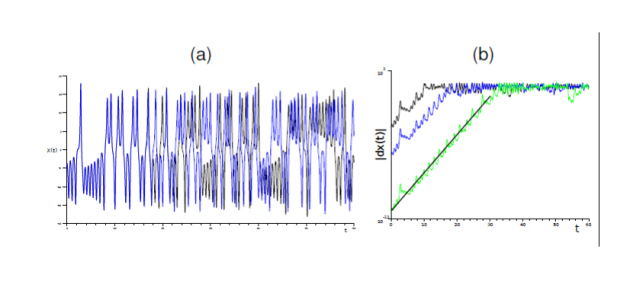
Note : Exponential growth of small errors
We observe an exponential increase of the maginutde of the disturbance
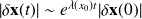
More specificaly, this exponential growth is in mean
So we obtain a rule in
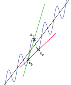
The analytical expression of the growth rate is done as
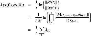
where we have used the chain rule
![]()
with the notation
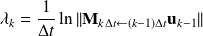
where
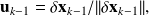 we have
From the experiment in Lorenz'63, the limit in n can exists and
is called the Lyapunov exponent. Note that since in finit dimension norms are equivalent, this expression does not depends on the norm used because of the limit of large time.
Warning :
But in finite time, the norm plays a role! (singular vector).
Conclusions
We need an initial condition to compute the time evolution by physical law
But, we can not observe the flow everywhere
Moreover, the flow is sensitive to initial conditions
Consequences
Since we cannot have access to the exact representation of the flow at a given time, the probabilistic approach is required.


