Temporal window
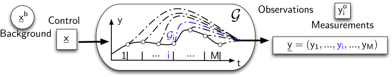
Control vector: \(\underline{x}=(x_1, ..., x_N)^T\)
Observations: \(\underline{y}^o=(y_1^o, ..., y_i^o, ..., y_M^o)^T\) at times \(i=1,..,\)
Generalized observation operator:
values \(\underline{y} = {\cal G}(\underline{x})= (y_1, ..., y_i, ..., y_M)^T\) simulated at times \(i=1,..,M\)
Cost function after choosing \(\underline{\underline B}\) and \(\underline{\underline R} =\hbox{diag}(R_1, ..., R_i, ... , R_M)\)
\(\displaystyle J(\underline{x}) ={1\over 2} \left(\underline{x} - \underline{x}^b\right)^T \underline{\underline B}^{-1} \left(\underline{x} - \underline{x}^b\right)+ {1\over 2} \sum_{i=1}^MR_i^{-1}\left[ y_i^o - {\cal G}_i (\underline{x}) \right]^2\)