
Basic concepts
Definition of an ”Analysis”
It is the process of estimating
The true state of a system at a given time
Possibly other model parameters
It is based on
Observational data (e.g. physical measurements)
A model of the physical system
Some ”a priori” information on the system
Possibly additional constraints (desired properties of the solution that are not present in the model)
A classical analysis method (Bertgthorson Doos, 1955)
Based on
Synchronous observations on-board ships (surface pressure)
Model parameters : temperature, wind and pressure
An evolution model defined on a spatial grid
This analysis was the following
Estimation of a first guess field obtained by extrapolation (time integration) of the model
Interpolation to get a predicted value at the observation location
Computation of the observed minus predicted quantities (a misfit)
Interpolation back on the model grid point of the misfit
Correction of the model parameters to reduce the misfit
This led to the optimal interpolation process still in use.
Wheather forecasts
In the domain of the numerical weather forecasting,
The analysis prepares intial conditions for weather forecasts
Observations of various types are available (data from satellites, ground stations, commercial flights, sounding balloons)
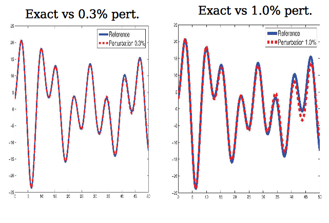
The discrepency between observed and predicted values is minimized : optimization problem
We will focus on the formulation and solution of the optimization problem. Note however that to have a rea- sonable solution, the data must be of a good quality in terms of coverage, and the models for the data have to be accurate.
An important problem : nonlinearity (I)
Solving a linear problem may be chalenging if it is large and/or very ill-conditioned
Nonlinearity introduces additional difficulties.
For instance on the Duffing's equation
 sensitivity with respect to initial conditions. Take for as truth
 ,
,
 and consider the perturbed conditions
 ,
,
 and
and
 ,
,
 .
.Comparison of the solutions obtained by time integration and interpret error in intial condition as analysis error.
The analysis error reduces the time period for which the forecast is close to the truth.
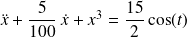
Perturbation of initial conditions : nonlinearity (II)
Until
 , the forecast seems reasonable with a
 perturbation
With a
 perturbation the two trajectories diverges already for

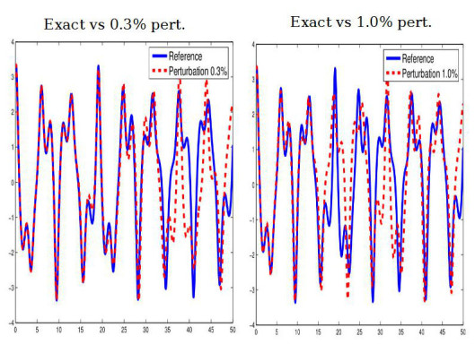
Perturbation of initial conditions : nonlinearity (III)
The reduction of the nonlinear term enlarges the time validity for the forecast
Angles to see Data Assimilation
The domain can be discussed from many angles :
Variational analysis
Optimization/Control theory
Estimation theory
Probability theory
Numerical optimization/linear algebra
High performance computing on parallel machines
Goal of this course show the connections between all this fields in the framework of Data Assimilation
Optimization point of view
Goal : find the initial state of a dynamical system to perform forecasts
Use observations and a model of the system
Determine the initial state by solving an optimization problem (here, a control problem). Minimize the
discrepancy between observations and model.
Parameter estimation view
A priori knowledge on values of

Observations :

Observation model
 + noise
Dynamical model
 + noise
 Find

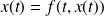
Estimation from set theory
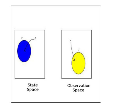
Estimation from set theory
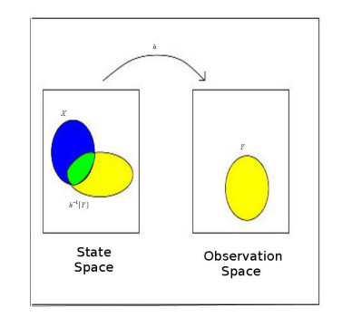
Inclusion of statistical knowledge
High performance computing point of view
The simplest instance of a Data Assimilation problem is a linear least squares problem
Typical sizes would be for this problem
 unknowns and
 observations (including a priori infomation)
The problem is not sparse
If no particular structure taken into account, the solution of the problem on a modern
 operations/s
computer would take 200 centuries of computation by the normal equations
In terms of memory, no available computer (2006) is able to store in core memory the matrix
Therefore parallel iterative methods are sought a are run on parallel computers


