Conclusion
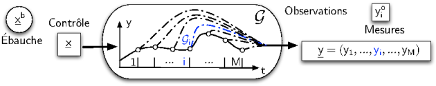
General cost function: \(\displaystyle J(\underline{x}) ={1\over 2} \left(\underline{x} - \underline{x}^b\right)^T \underline{\underline B}^{-1} \left(\underline{x} - \underline{x}^b\right)+ {1\over 2} \left[\underline{y}^o - {\cal G}(\underline{x})\right]^T \underline{\underline R}^{-1}\left[\underline{y}^o - {\cal G}(\underline{x})\right]\)
Descent methods imply the computation of the gradient of the cost function
When the observation operator is linear, one get the "BLUE" methods
In the nonlinear case, the incremental cost function approximates the cost function around the background state
The linearization of the observation operator can be approximated by finite differences
The 4D-Var method involves the computation of the adjoints of the evolution model with respect to initial contions